Lesson 4: Creating Your First Worksheet
To begin this lesson, open Microsoft Excel. You are now ready to start building your first worksheet. During this lesson you will review some things you have already learned and learn a few new things. The order in which you will complete the worksheet is not the most efficient. The exercises have been ordered to provide an opportunity to learn new skills and practice skills already learned. The lesson must be completed in the sequence presented. When you have completed all of the exercises, your worksheet will look like the one shown here.
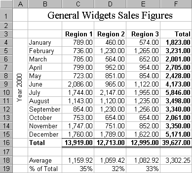
Let's start by entering the months of the year. You will use the Series function, which allows you to enter the first value in the series and have the computer enter the rest.
- Move the cursor to cell A1.
- Type January.
- Click on the checkmark located on the Formula bar. This will enter January into the cell. Clicking on the checkmark is similar to pressing Enter.

- Drag the Fill Handle (the small square located in the lower right corner of the cell) to cell A12. Point to the Fill Handle and hold down the left mouse button while you move the cursor down to cell A12. The months February through December should fill the cells.

Pressing the Num Lock key can make data entry easier. If you have a numeric keypad, Num Lock enables you to enter numbers as if you were using a calculator. You can also use the Enter key located on the numeric keypad. If you highlight the rows and columns into which you are going to enter data, the cursor will automatically move up and down those columns.
Enter the following values:
| A | B | C | D | |
| 1 | January | 789 | 460 | 574 |
| 2 | February | 736 | 1230 | 1265 |
| 3 | March | 785 | 564 | 652 |
| 4 | April | 799 | 952 | 954 |
| 5 | May | 723 | 851 | 854 |
| 6 | June | 2086 | 965 | 1122 |
| 7 | July | 1744 | 2147 | 1955 |
| 8 | August | 1143 | 1120 | 1235 |
| 9 | September | 854 | 1230 | 1256 |
| 10 | October | 753 | 654 | 654 |
| 11 | November | 1747 | 751 | 852 |
| 12 | December | 1760 | 1789 | 1622 |
- Highlight the area B1 to D12. Move the cursor to cell B1. Press F8. Press the down arrow key until you are in cell B12. Press the right arrow key until B1 to D12 are highlighted.
- Make sure Num Lock is on.
- Do NOT remove the highlighting.
- Type 789. Press Enter. You can use the Enter key located on the numeric keypad.
- Type 736. Press Enter.
- Type 785. Press Enter.
- Type 799. Press Enter.
- Type 723. Press Enter.
- Type 2086. Press Enter.
- Type 1744. Press Enter.
- Type 1143. Press Enter.
- Type 854. Press Enter.
- Type 753. Press Enter
- Type 1747. Press Enter.
- Type 1760. Press Enter. If the data area is still highlighted, the cursor will automatically move to cell C1.
- Type 460. Press Enter.
- Type 1230. Press Enter.
- Continue entering the data until you have entered it all.
- Press Esc when you have completed entering your data. Then click anywhere on the worksheet to remove the highlighting.
You can use Microsoft Excel to insert or delete rows on the worksheet. You need to insert three rows so you can add headings to the chart.
- Highlight cells A1 to A3. Move the cursor to cell A1. Press F8. Press the down arrow key twice.
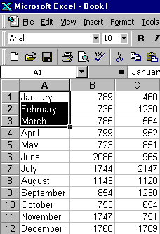
- Click on Insert, which is located on the Menu bar.
- Press the down arrow key until Rows is highlighted.
- Press Enter. Three new rows should be inserted.
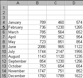
Creating a Series
You need to put headings on our columns of data. Use the Series function.
- Move the cursor to cell B3.
- Type Region 1.
- Click on the checkmark located on the Formula bar.
- Grab the Fill Handle and move the cursor right to cell D3. "Region 2" and "Region 3" should appear in cells C3 and D3, respectively.
Now right-align cells B3 to D3.
- Highlight cells B3 to D3.
- Click on the Align Right icon on the Formatting toolbar.

- Note the change in the text alignment
- Move the cursor to cell A16.
- Type Total.
- Press Enter.
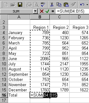
The AutoSum icon on the Standard toolbar automatically creates a SUM function. The following illustrates using the SUM function to total the Region 1 sales:
- Press F5.
- Type B16.
- Press Enter.
- Click on the AutoSum button, which is located on the Standard toolbar.

-
B4 to B15 should now be highlighted.
- Press Enter.
In Lesson Three you learned that you can copy and paste information. To copy the formula in cell B16 and paste it in cells C16 to D16, follow these steps:

Copy and Paste Icons
- Move to cell B16.
- Click on the Copy icon. Rotating dotted lines will appear around the cell. The rotating dotted lines designate the area to be copied.
- Highlight cells C16 to D16.
- Click on the Paste icon, which is located on the Standard toolbar. The formula in cell B16 is copied to cells C16 and D16.
- Press Esc.
Enter the word "Total" in cell E3 and right-align the cell.
- Move to cell E3.
- Type Total.
- Click on the checkmark located on the Formula bar.
- Click on the Align Right icon on the Formatting toolbar.
There is a Paste Function icon located on the Standard toolbar. You can use this icon to add a function to your worksheet. To sum the January sales figures:
- Move to cell E4.
- Click on the Paste Function icon on the Standard toolbar. The Paste Function dialog box opens.

- Click on Math & Trig in the Function Category box.
- Click on Sum in the Function Name box.
- Click on OK. The Function dialog box will open.
- Make sure that "B4:D4" displays in the Number 1 field. These are the fields that will be summed.
- Click on OK.
Copy the formula you just entered in cell E4 to cells E5 to E16.
- With your cursor in cell E4, click on the Copy icon on the Standard toolbar.
- Highlight cells E5 to E16.
- Click on the Paste icon.
- Press Esc and click anywhere on the worksheet to remove the highlighting.
Previously you learned how to center data within a cell. You can also center the data across several cells. The following illustrates:
- Move to cell A1.
- Type General Widgets Sales Figures.
- Press the Tab key.
- Highlight cells A1 to E1.
- Click on the Merge and Center icon.

Changing the Font and the Font Size
You can change the font and the font size of individual cells.
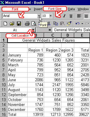
- Make sure the cursor is in A1. The title "General Widgets Sales Figures" is in cell A1.
- Click to open the Font drop down menu on the Formatting toolbar.
- Select Times New Roman.
- Move to the Font Size box, which is also located on the Formatting toolbar.
- Type 16.
- Press Enter.
You can use Microsoft Excel to insert or delete columns on the worksheet. You need to insert a column.
- Move the cursor to cell A4.
- Click on Insert, which is located on the Menu bar.
- Press the down arrow key until Columns is highlighted.
- Press Enter.
- A new column is inserted.
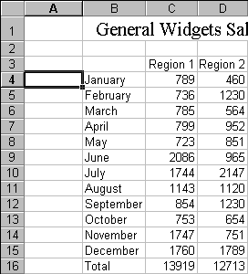
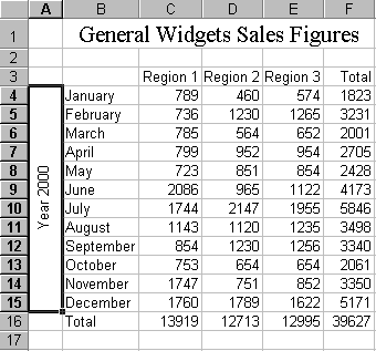
You can also align text sideways. After doing the following exercise, your worksheet should look like the illustration at the end of this exercise.
- Type Year 2000 in cell A4.
- Press Enter.
- Highlight A4 to A15.
- Click on Format, which is located on the Menu bar.
- Press the down arrow key until Cells is highlighted.
- Press Enter.
- Click on the Alignment tab, if it is not in the front.
- Select Center in the Horizontal field. This will center the text in the cell horizontally.
- Select Center in the Vertical field. This will center the text in the cell vertically.
- Click on the word "Text" in the Orientation frame. Set the orientation to 90 degrees. This will turn the text sideways.
- Select Merge Cells.
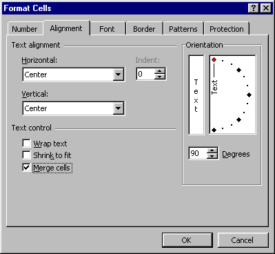
- Click on OK. The text now appears sideways as shown here.
Adding Text
Add the following text to your worksheet:
- Move the cursor to cell B18.
- Type Average.
- Press Enter.
- Type % of Total in cell B19.
- Press Enter.
Earlier in this lesson you learned about the Paste Function icon and how to use it to add a function to the worksheet. You can also use the Paste Function icon in the Point mode. When you are in the Point mode you can use your arrow keys or your mouse to select cells.
The following illustrates:
- Move the cursor to cell C18. You are going to enter a formula to calculate average regional sales for Region 1 in cell C18.
- Click on the Paste Function icon on the Standard toolbar. The paste function dialog box will open.

- Click on All in the Function Category box.
- Click on Average in the Function Name box.
- Click on OK.
- Move the Paste Function dialog box to the lower right corner of the screen so you can see the cells on the worksheet you will be working with.
- Highlight C4 to C15. Note that the lower right corner of the status bar reads "Point." This indicates that you are now in the point mode.
- Click on OK, in the Paste Function dialog box. The average sales for Region 1 should now appear in cell C18.
Copy the formula you just entered in cell C18 to cells D18 to F18. This will calculate the average sales for regions two and three and it will also calculate the average total sales.
- Move the cursor to cell C18.
- Press Ctrl-C. Pressing Ctrl-C selects the field to be copied.
- Press the right arrow key. You should be in cell D18.
- Highlight D18 to F18. Press F8. Press the right arrow key twice.
- Press Ctrl-V. This will paste the formula in cells D18 to F18.
- Press Esc.
- Click anywhere on the worksheet to clear the highlighting.
In this exercise you are going to enter a formula to calculate the regional sales as a percent of total sales and copy the resulting formula to cells D19 to E19. You will use the Point mode.
- Move the cursor to cell C19.
- Click on the Edit Formula icon (the equals sign) on the Formula bar. A dialog box will appear.

- Move the dialog box so that you can see your column headings. While holding down the left mouse button, drag the dialog box out of the way.
- Click in cell C16. C16, the numerator, will appear in cell C19.
- Press the slash.
- Click in cell F16. F16, the denominator, will appear in cell C19.
- Press F4 to make the cell address absolute.
- Click on the checkmark located on the Formula bar.
- Press Ctrl-C to copy the formula you just entered.
- Highlight D19 to E19. Move to cell D19. Press F8 anchor the cursor. Press the right arrow key.
- Press Ctrl-V to paste the formula in cells D19 and E19.
- Press Esc. You have finished copying.
Let�s bold the region names and the totals.
- Move the cursor to cell C3.
- Highlight cells C3 to F3.
- Click on the Bold icon, which is located on the Formatting toolbar.

- Highlight cells F4 to F16.
- Click on the Bold icon, which is located on the Formatting toolbar.
- Move the cursor to cell B16.
- Highlight cells B16 to F16.
- Click on the Bold icon again.
You can format your numbers to make them easier to read.
- Move the cursor to cell C4.
- Highlight cells C4 to F18.
- Click on Format, which is located on the Menu bar.
- Press the down arrow key until Cells is highlighted.
- Press Enter.
- Click on the Number tab, if it is not in the front.
- Click on Number in the Category box.
- Type 2 in the Decimal Places field. This will cause the number to display with two decimal places.
- Place a checkmark in the Use 1000 Separator box. This will cause thousands to be separated with a comma.
- Click on OK to close the dialog box.
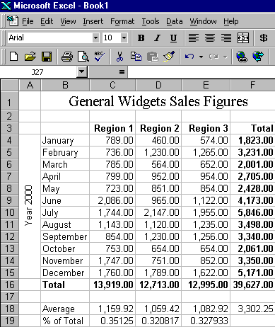
Your worksheet should look similar to the one shown here.
You can use the Border icon to place borders around a cell. You have several options on the type of border to use and where to place the borders. Borders can be placed above, below, and/or on the sides of cells. The following illustrates using borders:
- Place the cursor in cell C16.
- Highlight cells C16 to F16.
- Click on the down arrow next to the Borders icon to open the Borders palette.

- Click on Top and Double Bottom Border (farthest right in the middle row).

In Lesson Three you learned how to format a number as a percent by using the icon on the toolbar. You can also format a number as a percent by using the menu. The following illustrates:
- Highlight cells C19 to E19.
- Click on Format, which is located on the Menu bar.
- Press the down arrow until Cells is highlighted.
- Press Enter.
- Click on the Number tab, if it is not in the front.
- Click on Percent in the Category box.
- Type 0 in the Decimal Places field. This will cause the number to display with no decimal places.
- Click on OK.

Your worksheet is complete. It should look similar to the one shown here.
You have completed your first worksheet. You are now ready to print it. First, look at the worksheet in the Print Preview screen.
- Click on File, which is located on the Menu bar.
- Press the down arrow key until Print Preview is highlighted.
- Press Enter. The worksheet as it will appear when printed should display.
- Click on Setup.
- Select Portrait on the Page tab.
- Click on the Margin tab.
- Place a checkmark in the Center on Page Horizontally box.
- Click on OK.
- Click on Print. A dialog box will appear.
- Check the setting in the dialog box.
- Click on OK.
This is the end of Lesson Four. Save your file and close Microsoft Excel.
- Click on File, which is located on the Menu bar.
- Press the down arrow key until Save is highlighted.
- Press Enter.
- Type lesson4.xls in the filename field.
- Click on Save.
- Click on File, which is located on the Menu bar.
- Press the down arrow key until Exit is highlighted.
- Press Enter.
