Lesson 1: Getting Familiar with Microsoft Excel

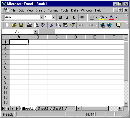
This course teaches Microsoft Excel basics. Although knowledge of how to navigate in a Windows environment is helpful, this course was created for the computer novice. To begin, open Microsoft Excel. The screen shown here will appear.

The Title Bar

This lesson will familiarize you with the Microsoft Excel screen. We will start with the Title bar, which is located at the very top of the screen. On the Title bar, Microsoft Excel displays the name of the workbook you are currently using. At the top of your screen, you should see "Microsoft Excel - Book1" or a similar name.

The Menu Bar

The Menu bar is directly below the Title bar and displays the menu. The menu begins with the word File and continues with the following: Edit, View, Insert, Format, Tools, Data, Window, and Help. You use the menu to give instructions to the software. Point with your mouse to a menu option and click the left mouse button. A drop-down menu will appear. You can now use the left and right arrow keys on your keyboard to move left and right across the Menu bar options. You can use the up and down arrow keys to move up and down the drop-down menu. To select an option, highlight the item on the drop-down menu and press Enter. An ellipse after a menu item signifies additional options; if you select that option, a dialog box will appear.

Do the following exercise, which demonstrates using the Microsoft Excel menu.

1. Point to the word File, which is located on the Menu bar.
2. Click your left mouse button.
3. Press the right arrow key until Help is highlighted.
4. Press the left arrow key until Format is highlighted.
5. Press the down arrow key until Style is highlighted.
6. Press the up arrow key until Cells is highlighted.
7. Press Enter to select the Cells menu option.
8. Point to Cancel and click the left mouse button to close the dialog box.

Toolbars provide shortcuts to menu commands. Toolbars are generally located just below the Menu bar. Before proceeding with the lesson, make sure the toolbars we will use -- Standard and Formatting -- are available. Follow the steps outlined here:

1. Point to View, which is located on the Menu bar.
2. Click the left mouse button.
3. Press the down arrow key until Toolbars is highlighted.
4. Press Enter. Both Standard and Formatting should have a checkmark next to them. If both have a checkmark next to them, press Esc three times to close the menu. If either does not have a checkmark, press the down arrow key until Customize is highlighted.
5. Press Enter.
6. Point to the box or boxes next to the unchecked word or words, Standard and/or Formatting, and click the left mouse button. A checkmark should appear.
7. Note: You turn the checkmark on and off by clicking the left mouse button.
8. Point to Close and click the left mouse button to close the dialog box.

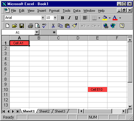
Microsoft Excel consists of worksheets. Each worksheet contains columns and rows. The columns are lettered A to IV; the rows are numbered 1 to 65536. The combination of column and row coordinates make up a cell address. For example, the cell located in the upper left corner of the worksheet is cell A1, meaning column A, row 1. Cell E10 is located under column E on row 10. You enter your data into the cells on the worksheet.

The Formula Bar

If the Formula bar is turned on, the cell address displays on the left side of the Formula bar. Cell entries display on the right side of the Formula bar. Before proceeding, make sure the Formula bar is turned on.

1. Point to View, which is located on the Menu bar.
2. Click the left mouse button. A drop-down menu will appear.
3. On the drop-down menu, if Formula Bar has a checkmark next to it, the Formula bar is turned on. Press the Esc key twice to close the drop-down menu.
4. If Formula Bar does not have a checkmark next to it, press the down arrow key until Formula Bar is highlighted and press Enter. The Formula bar should appear below the toolbars.
5. Note that the current cell address displays on the left side of the Formula bar.

If the Status bar is turned on, it appears at the very bottom of the screen. Before proceeding, make sure the Status bar is turned on.

1. Point to View, which is located on the Menu bar.
2. Click the left mouse button. A drop-down menu will appear.
3. On the drop-down menu, if Status Bar has a checkmark next to it, it is turned on. Press the Esc key twice to close the drop-down menu.
4. If Status Bar does not have a checkmark next to it, press the down arrow key until Status Bar is highlighted and press Enter. The Status bar should appear at the bottom of the screen.

The Num Lock key is a toggle key. Pressing it turns the numeric keypad on and off. You can use the numeric keypad to enter numbers as if you were using a calculator. The letters "NUM" on the Status bar in the lower right corner of the screen indicate that the numeric keypad is on.

1. Press the Num Lock key several times and note how the indicator on the Status bar changes.
2. The Caps Lock key is also a toggle key. Pressing it turns the caps function on and off. When the caps function is on, your entry will appear in capital letters.
3. Press the Cap Lock key several times and note how the indicator on the Status bar changes.

Make sure the Scroll Lock and End indicators are off and complete the following exercises.

The Down Arrow Key

You can use the down arrow key to move downward on the screen one cell at a time.

1. Press the down arrow key several times.
2. Note that the cursor moves downward one cell at a time.

You can use the Up Arrow key to move upward on the screen one cell at a time.

1. Press the up arrow key several times.
2. Note that the cursor moves upward one cell at a time.

You can use the right and left arrow keys to move right or left one cell at a time.

1. Press the right arrow key several times.
2. Note that the cursor moves to the right.
3. Press the left arrow key several times.
4. Note that the cursor moves to the left.

The Page Up and Page Down keys move the cursor up and down one page at a time.

1. Press the Page Down key.
2. Note that the cursor moves down one page.
3. Press the Page Up key.
4. Note that the cursor moves up one page.

The End key, used in conjunction with the arrow keys, causes the cursor to move to the far end of the spreadsheet in the direction of the arrow.

1. Press the End key.
2. Note that "END" appears on the Status bar in the lower right corner of the screen.
3. Press the right arrow key.
4. Note that the cursor moves to the farthest right area of the screen.
5. Press the END key again.
6. Press the down arrow key. Note that the cursor moves to the bottom of the screen.
7. Press the End key again.
8. Press the left arrow key. Note that the cursor moves to the farthest left area of the screen.
9. Press the End key again.
10. Press the up arrow key. Note that the cursor moves to the top of the screen.

The Home Key

The Home key, used in conjunction with the End key, moves you to cell A1 -- or to the beginning of the data area if you have entered data.

1. Move the cursor to column J.
2. Stay in column J and move the cursor to row 20.
3. Press the End key.
4. Press Home.
5. You should now be in cell A1.

Scroll Lock moves the window, but not the cell pointer.

1. Press the Page Down key.
2. Press Scroll Lock. Note "SCRL" appears on the Status bar in the lower right corner of the screen.
3. Press the up arrow key several times. Note that the cursor stays in the same position and the window moves upward.
4. Press the down arrow key several times. Note that the cursor stays in the same position and the window moves downward.
5. Press Scroll Lock to turn the scroll lock function off.
6. Press End.
7. Press Home. You should be in cell A1.

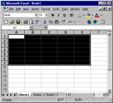
If you wish to perform a function on a group of cells, you must first select those cells by highlighting them. To highlight cells A1 to E1:

1. Place the cursor in cell A1.
2. Press the F8 key. This anchors the cursor.
3. Note that EXT appears on the Status bar in the lower right corner of the screen. You are in the Extend mode.
4. Click in cell E7. Cells A1 to E7 should now be highlighted.
5. Press Esc and click anywhere on the worksheet to clear the highlighting.

You can also highlight an area by holding down the left mouse button and dragging the mouse over the area. In addition, you can select noncontiguous areas of the worksheet by doing the following:

1. Place the cursor in cell A1.
2. Hold down the Ctrl key. Do not release it until you are told. Holding down the Ctrl key enables you to select noncontiguous areas of the worksheet.
3. Press the left mouse button.
4. While holding down the left mouse button, use the mouse to move from cell A1 to E7.
5. Continue to hold down the Ctrl key, but release the left mouse button.
6. Using the mouse, place the cursor in cell G8.
7. Press the left mouse button.
8. While holding down the left mouse button, move to cell I17. Release the left mouse button.
9. Release the Ctrl key.
10. Press Esc and click anywhere on the worksheet to remove the highlighting.

This is the end of Lesson One. Close Microsoft Excel.

1. Click on File, which is located on the Menu bar.
2. Press the down arrow key until Exit is highlighted.
3. Press Enter.
4. Click on No, if you are prompted, "Do you want to save the changes you made to Book1?"