
Lesson 2: Formatting Text and Performing Mathematical Calculations
In this lesson, you are going to learn how to format text and perform basic mathematical calculations. To start, open a blank Microsoft Excel workbook.
Choosing a Default Font
Microsoft Excel enables you to choose a default font. The default font is the style of typeface that Excel will use unless you specify a different style. For the exercises in this lesson, you want your font to be set to Arial, Regular, and Size 10. To set your font to Arial, Regular, and Size 10:
- Choose Format > Cells from the menu.
- Choose the Font tab.
- In the Font box, choose Arial.
- In the Font Style box, choose Regular.
- In the Size box, choose 10.
- If there is no check mark in the Normal Font box, click to place a check mark there. Your selections are now the default.
- Click OK.
Adjusting the Standard Column Width
When you open Microsoft Excel, the width of each cell is set to a default width. This width is called the standard column width. You need to change the standard column width to complete your exercises. To make the change, follow these steps:
- Choose Format > Column > Standard Width from the menu. The Standard Width dialog box opens.
- Type 25 in the Standard Column Width field. Click OK. The width of every cell on the worksheet should now be set to 25.
- Move to cell A1.
- Type Cathy.
- Press Enter.
Cell Alignment
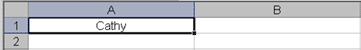
The name "Cathy" is aligned with the left side of the cell. You can change the cell alignment.
![]()
Centering by Using the Menu
To center the name Cathy, follow these steps:
- Move the cursor to cell A1.
- Choose Format > Cells from the menu. The Format Cells dialog box opens.
- Choose the Alignment tab.
- Click to open the drop-down box associated with the Horizontal field. After the drop-down box is opened, click Center.
- Click OK to close the dialog box. The name "Cathy" is centered.
Right-Aligning by Using the Menu
To right-align the name "Cathy," follow these steps:
- Move the cursor to cell A1.
- Choose Format > Cells from the menu. The Format Cells dialog box opens.
- Choose the Alignment tab.
- Click to open the drop-down box associated with the Horizontal field. After the drop-down box opens, click Right (Indent).
- Click OK to close the dialog box. The name "Cathy" is right-aligned.
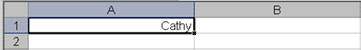
Left-Aligning by Using the Menu
To left-align the name "Cathy," follow these steps:
- Move the cursor to cell A1.
- Choose Format > Cells from the menu. The Format Cells dialog box opens.
- Choose the Alignment tab.
- Click to open the drop-down box associated with the Horizontal field. After the drop-down box opens, click Left (Indent).
- Click OK to close the dialog box. The name "Cathy" is left-aligned.
![]()
Alternate Method: Alignment by Using the Formatting Toolbar
Using the Formatting toolbar, you can quickly perform tasks. You can use the Formatting toolbar to change alignment.
Centering by Using the Toolbar
To center the name "Cathy," follow these steps:
- Move the cursor to cell A1.
- Click the Center icon, which is located on the Formatting toolbar.
![]()
The red circle designates the Align Center icon.
Right-Aligning by Using the Toolbar
You can right-align the name "Cathy" by following these steps:
- Move the cursor to cell A1.
- Click the Align Right icon, which is located on the Formatting toolbar.
![]()
The red circle designates the Align Right icon.
Left-Aligning by Using the Toolbar
You can left-align the name "Cathy" by following these steps:
- Move the cursor to cell A1.
- Click the Align Left icon, which is located on the Formatting toolbar.
![]()
The red circle designates the Align Left icon.
Adding Bold, Underline, and Italic
You can bold, underline, or italicize text in Microsoft Excel. You can also combine these features -- in other words, you can bold, underline, and italicize a single piece of text.
In the exercises that follow, you will learn three different methods for bolding, italicizing, or underlining text in Microsoft Excel. You will learn to bold, italicize, and underline by using the menu, the icons, and the shortcut keys.
Adding Bold by Using the Menu
- Type Bold in cell A2.
- Click the check mark located on the Formula bar. Clicking on the check mark is similar to pressing Enter.
- Choose Format > Cells from the menu. The Format Cells dialog box opens.
- Choose the Font tab.
- Click Bold in the Font Style box.
- Click OK. The word "Bold" should now be bolded.
Adding Italic by Using the Menu
- Type Italic in cell B2.
- Click the check mark located on the Formula bar. Clicking on the check mark is similar to pressing Enter.
- Choose Format > Cells from the menu. The Format Cells dialog box opens.
- Click Italic in the Font style box.
- Click OK. The word "Italic" is italicized.
Adding Underline by Using the Menu
Microsoft Excel provides several types on underlines. The exercise that follows illustrates some of them.
Single Underline
- Type Underline in cell C2.
- Click the check mark located on the Formula bar. Clicking on the check mark is similar to pressing Enter.
- Choose Format > Cells from the menu. The Format Cells dialog box opens.
- Click to open the drop-down menu associated with the Underline box.
- Click Single.
- Click OK. The cell entry now has a single underline.
Double Underline
- Type Underline in cell D2.
- Click the check mark located on the Formula bar.
- Choose Format > Cells from the menu. The Format Cells dialog box opens.
- Click to open the drop-down menu associated with the Underline field.
- Click Double.
- Click OK. The cell entry now has a double underline.
Single Accounting
- Type Underline in cell E2.
- Click the check mark located on the Formula bar.
- Choose Format > Cells from the menu. The Format Cells dialog box will open.
- Click to open the drop-down menu associated with the Underline field.
- Click Single Accounting.
- Click OK. The cell entry now has a single accounting underline.
Double Accounting
- Type Underline in cell F2.
- Click the check mark located on the Formula bar.
- Choose Format > Cells from the menu. The Format Cells dialog box will open.
- Click to open the drop-down menu associated with the Underline field.
- Click Double Accounting.
- Click OK. The cell entry now has a double accounting underline.
Adding Bold, Underline, and Italic by Using the Menu
- Move the cursor to cell G3.
- Type All three.
- Click the check mark located on the Formula bar.
- Choose Format > Cells from the menu. The Format Cells dialog box opens.
- Choose the Font tab.
- Click Bold Italic in the Font Style box.
- Click to open the drop-down menu associated with the Underline field. Then click Single.
- Click OK. The words "All three" are now bolded, italicized, and underlined.
Removing Bolding and Italics by Using the Menu
- Highlight cells A2 to B2. Place your cursor in cell B2. Press the F8 key. Press the right arrow key once.
- Choose Format > Cells from the menu. The Format Cells dialog box opens.
- Click Regular in the Font style box.
- Click OK. Cell A2 is no longer be bolded. Cell B2 is no longer italized.
Removing an Underline by Using the Menu
- Move to cell C2.
- Choose Format > Cells from the menu. The Format Cells dialog box opens.
- Click to open the drop-down menu associated with the Underline field. Then click None.
- Click OK. The underdelined is removed.
Alternate Method: Adding Bold by Using the Icon
- Type Bold in cell A3.
- Click the check mark located on the Formula bar.
![]()
- Click the Bold icon, which is on the Formatting toolbar.
- Click again on the Bold icon if you wish to remove the bolding.
Alternate Method: Adding Italic by Using the Icon
- Type Italic in cell B3.
- Click the check mark located on the Formula bar.
![]()
- Click the Italic icon, which is on the Formatting toolbar.
- Click again on the Italic icon if you wish to remove the italics.
Alternate Method: Adding Underline by Using the Icon
- Type Underline in cell C3.
- Click the check mark located on the Formula bar.
![]()
- Click the Underline icon, which is on the Formatting toolbar.
- Click again on the Underline icon if you wish to remove the underline.
Alternate Method: Adding Bold, Underline, and Italic by Using Icons
- Type All Three in cell D3.
- Click the check mark located on the Formula bar.
- Click the Bold icon.
- Click the Italic icon.
- Click the Underline icon.
Alternate Method: Adding Bold by Using Shortcut Keys
- Type Bold in cell A4.
- Click the check mark located on the Formula bar.
- Hold down the Ctrl key while pressing "b" (Ctrl-b).
- Press Ctrl-b again if you wish to remove the bolding.
Alternate Method: Adding Italic by Using Shortcut Keys
- Type Italic in cell B4.
- Click the check mark located on the Formula bar.
- Hold down the Ctrl key while pressing "i" (Ctrl-i).
- Press Ctrl-i again if you wish to remove the italic formatting.
Alternate Method: Adding Underline by Using Shortcut Keys
- Type Underline in cell C4.
- Click the check mark located on the Formula bar.
- Hold down the Ctrl key while pressing "u" (Ctrl-u).
- Press Ctrl-u again, if you wish to remove the underline.
Alternate Method: Adding Bold, Underline, and Italic by Using Shortcut Keys
- Type All three in cell D4.
- Click the check mark located on the Formula bar.
- Hold down the Ctrl key while pressing "b" (Ctrl-b).
- Hold down the Ctrl key while pressing "i" (Ctrl-i).
- Hold down the Ctrl key while pressing "u" (Ctrl-u).
Changing the Font, Font Size, and Font Color
You can change the Font, Font Size, and Font Color of the data you enter.
Changing the Font
- Type Times New Roman in cell A5.
- Click the check mark located on the Formula bar.
- Choose Format > Cells from the menu. The Format Cells dialog box opens.
- Choose the Font tab. All of the Fonts listed in the Font box are available to you.
- Find and click Times New Roman in the Font box.
- Click OK. The font changes from Arial to Times New Roman.
Changing the Font Size
- Place the cursor in cell A5.
- Choose Format > Cells from the menu. The Format Cells dialog box opens.
- Choose the Font tab.
- Click 16 in the Size box.
- Click OK. The font size changes to 16.
Changing the Font Color
- Place the cursor in cell A5.
- Choose Format > Cells from the menu. The Format Cells dialog box opens.
- Choose the Font tab.
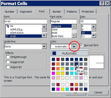
- Click to open the drop-down menu associated with the color field.
- Click Blue.
- Click OK. The font color changes to blue.
Alternate Method: Changing the Font Color by Using the Icon
- Place the cursor in cell A5.
- Click the down arrow next to the Font Color icon.
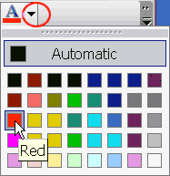
- Click on Red. Your font color changes to red.
Working with Long Text
Whenever you type text that is too long to fit into a cell, Microsoft Excel attempts to display all the text. It left-aligns the text regardless of the alignment that has been assigned to it, and it borrows space from the blank cells to the right. However, a long text entry will never write over cells that already contain entries -- instead, the cells that contain entries cuts off the long text. Do the following exercise to see how this works.
- Move the cursor to cell A6.
- Type Now is the time for all good men to go to the aid of their army.
- Press Enter. Everything that does not fit into cell A6 spills over into the adjacent cell.
- Move the cursor to cell B6.
- Type TEST.
- Press Enter. The entry in cell A6 is cut off.
- Move the cursor to cell A6.
- Look at the Formula bar. The text is still in the cell.
Changing a Single Column Width
Earlier you increased the column width of every column on the worksheet. You can also increase individual column widths. If you increase the column width, you will be able to see the long text.
- Make sure the cursor is anywhere under column A.
- Choose Format > Column > Width from the menu. The column width dialog box opens.
- Type 55 in the Column Width field.
- Click OK.
Column A is set to a width of 55. You should now be able to see all of the text.
Alternate Method: Changing a Single Column Width by Dragging
You can also change the column width with the cursor.
- Place the cursor on the line between the B and C column headings. The cursor should look like the one displayed here, with two arrows.
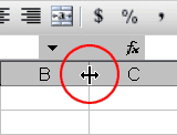
- Move your mouse to the right while holding down the left mouse button. The width indicator appears on the screen.
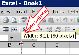
- Release the left mouse button when the width indicator shows approximately 40.
Moving to a New Worksheet
In Microsoft Excel, each workbook is made up of several worksheets. Before moving to the next topic, move to a new worksheet.
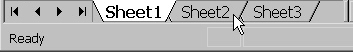
- Click Sheet2 in the lower left corner of the screen.
Setting the Enter Key Direction
In Microsoft Excel, you can specify which direction the cursor moves when you press the Enter key. You can have the cursor move up, down, left, right, or not at all. You will now make sure the cursor is set to move down when you press the Enter key.
- Choose Tools > Options from the menu. The Options dialog box opens.
- Choose the Edit tab.
- Make sure there is a check mark in the "Move Selection after Enter" box.
- If Down is not selected, click to open the Direction drop-down box. Click Down.
- Click OK.
Making Numeric Entries
In Microsoft Excel, you can enter numbers and mathematical formulas into cells. When a number is entered into a cell, you can perform mathematical calculations such as addition, subtraction, multiplication, and division. When entering a mathematical formula, precede the formula with an equal sign. Use the following to indicate the type of calculation you wish to perform:
+ Addition
- Subtraction
* Multiplication
/ Division
^ Exponential
Performing Mathematical Calculations
The following exercises demonstrate how to perform mathematical calculations.
Addition
- Move your cursor to cell A1.
- Type 1.
- Press Enter.
- Type 1 in cell A2.
- Press Enter.
- Type =A1+A2 in cell A3.
- Press Enter. Cell A1 has been added to cell A2, and the result is shown in cell A3.
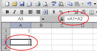
Place the cursor in cell A3 and look at the Formula bar.
Subtraction
- Press F5. The Go To dialog box opens.
- Type B1 in the Reference field.
- Press Enter. The cursor should move to cell B1.
- Type 5 in cell B1.
- Press Enter.
- Type 3 in cell B2.
- Press Enter.
- Type =+B1- B2 in cell B3.
- Press Enter. Cell B1 has been subtracted from B2, and the result is shown in cell B3.
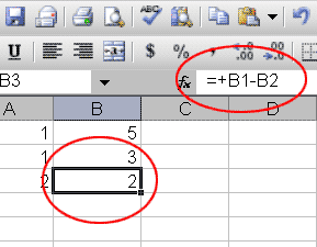
Place the cursor in cell B3 and look at the Formula bar.
Multiplication
- Hold down the Ctrl key while you press "g" (Ctrl-g). The Go To dialog box opens.
- Type C1 in the Reference field.
- Press Enter. You should now be in cell C1.
- Type 2 in cell C1.
- Press Enter.
- Type 3 in cell C2.
- Press Enter.
- Type =C1*C2 in cell C3.
- Press Enter. Cell C1 is multiplied by cell C2 and the result is displayed in cell C3.
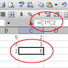
Place the cursor in cell C3 and look at the Formula bar.
Division
- Press F5.
- Type D1 in the Reference field.
- Press Enter. You should now be in cell D1.
- Type 6 in cell D1.
- Press Enter.
- Type 3 in cell D2.
- Press Enter.
- Type =D1/D2 in cell D3.
- Press Enter. Cell D1 is divided by cell D2 and the result is displayed in cell D3.
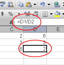
Place the cursor in cell D3 and look at the Formula bar.
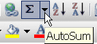
The AutoSum Icon
The AutoSum icon on the Standard toolbar automatically adds a column of numbers. The following illustrates the SUM function:
- Go to cell F1.
- Type 3. Press Enter.
- Type 3. Press Enter.
- Type 3. Press Enter.
- Click the AutoSum button, which is located on the Standard toolbar.
- F1 to F3 should now be highlighted.
- Press Enter. Cells F1 through F3 are added.
Automatic Calculation
If you have automatic calculation turned on, Microsoft Excel recalculates the worksheet as you change cell entries. You can check to make sure automatic calculation is turned on.
Setting Automatic Calculation
- Choose Tools > Options from the menu.
- Choose the Calculation tab.
- Select Automatic if it is not already selected.
- Click OK.
Trying Automatic Calculation
Make the changes outlined below and note how Microsoft Excel automatically recalculates.
- Move to cell A1.
- Type 2. Press the Enter key. The results shown in cell A3 have changed. The number in cell A1 has been added to the number in cell A2 and the results display in cell A3.
- Move to cell B1.
- Type 6.
- Press the Enter key. The results shown in cell B3 have changed. The number in cell B1 has been subtracted from the number in cell B2 and the results display in cell B3.
- Move to cell C1.
- Type 4. Press the Enter key. The results shown in cell C3 have changed. The number in cell C1 has been multiplied by the number in cell C2 and the results display in cell C3.
- Move to cell D1.
- Type 12. Press the Enter key. The results shown in cell D3 have changed. The number in cell D1 has been divided by the number in cell D2 and the results display in cell D3.
Formatting Numbers
You can format the numbers you enter into Microsoft Excel. You can add commas to separate thousands, specify the number of decimal places, place a dollar sign in front of the number, or display the number as a percent in addition to several other options.
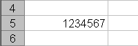
Before formatting
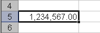
After formatting
- Move the cursor to cell A5.
- Type 1234567.
- Press Enter.
- Move the cursor back to cell A5.
- Choose Format > Cells from the menu. The Format Cells dialog box will open.
- Choose the Number tab.
- Click Number in the Category box.
- Type 2 in the Decimal Places box.
- Place a check mark in the Use 1000 Separator box.
- Click OK. The number should now display with two decimal places. The thousands should now be separated by commas.
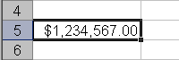
Adding a Dollar Sign to a Numeric Entry
- Move the cursor to cell A5.
- Choose Format > Cells from the menu. The Format Cells dialog box opens.
- Choose the Number tab.
- Click Currency in the Category box.
- Make sure there is a "$" in the Symbol box.
- Click OK. The number displays with a dollar sign.
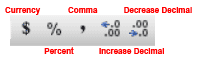
Alternate Method: Formatting Numbers by Using the Toolbar
- Move the cursor to cell A6.
- Type 1234567.
- Press Enter.
- Move the cursor back to cell A6.
- Click twice on the Increase Decimal icon to change the number format to two decimal places. Clicking on the Decrease Decimal icon decreases the decimal places.
- Click once on the Comma Style icon to add commas to the number.
- To change the number to a currency format, click Currency Style format.
- Move the cursor to cell A7.
- Type .35 (note the decimal point).
![]()
- Press Enter.
- Move the cursor back to cell A7.
- Click the Percent Style icon to turn .35 to a percent.
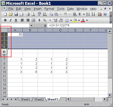
More Advanced Mathematical Calculations
When you perform mathematical calculations in Microsoft Excel, be careful of precedence. Calculations are performed from left to right, with multiplication and division performed before addition and subtraction.
- Move to a new worksheet by clicking on Sheet3 in the lower left corner of the screen.
- Go to cell A1.
- Type =3+3+12/2*4.
- Press Enter.
Note: Microsoft Excel divided 12 by 2, multiplied the answer by 4, added 3, and then added another 3. The answer, 30, displays in cell A1.
To change the order of calculation, use parentheses. Microsoft Excel calculates the information in parentheses first.
- Double-click in cell A1.
- Edit the cell to read =(3+3+12)/2*4.
- Press Enter.
Note: Microsoft Excel added 3 plus 3 plus 12, divided the answer by 2, and multiplied the result by 4. The answer, 36, displays in cell A1.
Cell Addressing
Microsoft Excel records cell addresses in formulas in three different ways, called absolute, relative, and mixed. The way a formula is recorded is important when you copy it.
With relative cell addressing, when you copy a formula from one area of the worksheet to another, Microsoft Excel records the position of the cell relative to the cell that originally contained the formula. The following exercises demonstrate:
- Go to cell A7.
- Type 1. Press Enter.
- Type 1. Press Enter.
- Type 1. Press Enter.
- Go to cell B7.
- Type 2. Press Enter.
- Type 2. Press Enter.
- Type 2. Press Enter.
- Go to cell A10.
In addition to typing a formula, as you did in Lesson 1, you can also enter formulas by using Point mode. When you are in Point mode, you can enter a formula either by clicking on a cell with your mouse or by using the arrow keys.
- You should be in cell A10.
- Type =.
- Use the up arrow key to move to cell A7.
- Type +.
- Use the up arrow key to move to cell A8.
- Type +.
- Use the up arrow key to move to cell A9.
- Press Enter.
- Look at the Formula bar while in cell A10. Note that the formula you entered is recorded in cell A10.
Copying by Using the Menu
You can copy entries from one cell to another cell. To copy the formula you just entered, follow these steps:
- You should be in cell A10.
- Choose Edit > Copy from the menu. Moving dotted lines appear around cell A10, indicating the cells to be copied.
- Press the Right Arrow key once to move to cell B10.
- Choose Edit > Paste from the menu. The formula in cell A10 is copied to cell B10.
- Press Esc to exit the Copy mode.
Compare the formula in cell A10 with the formula in cell B10 (while in the respective cell, look at the Formula bar). The formulas are the same except that the formula in cell A10 sums the entries in column A and the formula in cell B10 sums the entries in column B. The formula was copied in a relative fashion.
Before proceeding with the next exercise, you must copy the information in cells A7 to B9 to cells C7 to D9. This time you will copy by using the Formatting toolbar.
Copying by Using the Formatting Toolbar
- Highlight cells A7 to B9. Place the cursor in cell A7. Press F8. Press the down arrow key twice. Press the right arrow key once. A7 to B9 should be highlighted.
- Click the Copy icon
 ,
which is located on the Formatting toolbar.
,
which is located on the Formatting toolbar. - Use the arrow key to move the cursor to cell C7.
- Click the Paste icon
 ,
which is located on the Formatting toolbar.
,
which is located on the Formatting toolbar. - Press Esc to exit Copy mode.
Absolute Cell Addressing
An absolute cell address refers to the same cell, no matter where you copy the formula. You make a cell address an absolute cell address by placing a dollar sign in front of both the row and column identifiers. You can do this automatically by using the F4 key. To illustrate:
- Move the cursor to cell C10.
- Type =.
- Use the up arrow key to move to cell C7.
- Press F4. Dollar signs should appear before the C and before the 7.
- Type +.
- Use the up arrow key to move to cell C8.
- Press F4.
- Type +.
- Use the up arrow key to move to cell C9.
- Press F4.
- Press Enter. The formula is recorded in cell C10.
Copying by Using the Keyboard Shortcut
Now copy the formula from C10 to D10. This time, you will copy by using the keyboard shortcut.
- Your cursor should be in cell C10.
- Hold down the Ctrl key while you press "c" (Ctrl-c). This copies the contents of cell C10.
- Press the right arrow once.
- Hold down the Ctrl key while you press "v" (Ctrl-v). This pastes the contents of cell C10 in cell D10.
- Press Esc to exit the Copy mode.
Compare the formula in cell C10 with the formula in cell D10. They are the same. The formula was copied in an absolute fashion. Both formulas sum column C.
Mixed Cell Addressing
You use mixed cell addressing to reference a cell that is part absolute and part relative. You can use the F4 key.
- Move the cursor to cell E1.
- Type =.
- Press the up arrow key once.
- Press F4.
- Press F4 again. Note that the column is relative and the row is absolute.
- Press F4 again. Note that the column is absolute and the row is relative.
- Press Esc.
Deleting Columns
You can delete columns from your spreadsheet. To delete columns C and D:
- Click on column C and drag to column D.
- Choose Edit > Delete from the menu. Column D is deleted.
- Click anywhere on the spreadsheet to remove your selection.
Deleting Rows
You can delete rows from your spreadsheet. To delete rows 1 through 4:
- Click the row 1 and drag to row 4.
- Choose Edit > Delete from the menu. Rows 1 through 4 are deleted.
- Click anywhere on the spreadsheet to remove your selection.
Inserting Columns
There will be times when you will need to insert a column or columns into your spreadsheet. To insert a column:
- Click on A to select column A.
- Choose Insert > Columns from the menu. A column is inserted to the right of column A.
- Click anywhere on the spreadsheet to remove your selection.
Inserting Rows
You can also insert rows into your spreadsheet:
- Click on 2 to select row 2.
- Choose Insert > Rows from the menu. A row is inserted above row 2.
- Click anywhere on the spreadsheet to remove your selection.
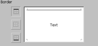
Creating Borders
You can use borders to make entries on your spreadsheet stand out. Accountants usually place a single underline above a final number and a double underline below. The following illustrates:
- Go to cell B7.
- Choose Format > Cells from the menu.
- Choose the Border tab.
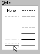
- In the Style box, click on the single underline.
- Click the top of the Border box.
- In the Style box, click on the double underline.
- Click the bottom of the Border box.
- Click OK. Cell B7 now has a border.
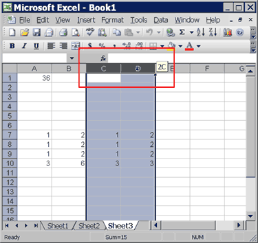
Alternate Method: Creating Borders by Using the Icon
- Go to cell C7. Click the down arrow beside the Borders icon.
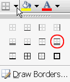
- Select the Top and Double Bottom Border. Cell C7 now has borders.
Merge and Center
You will sometimes want to center a piece of text over several columns. The following example shows you how.
- Go to cell B1.
- Type Sample Spreadsheet.
- Click the check mark on the Formula bar.
- Select columns B1 to D1.
- Click the Merge and Center icon
 on
the formatting toolbar. Cells B1, C1, and D1 are merged and centered.
on
the formatting toolbar. Cells B1, C1, and D1 are merged and centered.
Adding Background Color
You can add background color to a cell or group of cells:
- Go to cell B1.
- Choose Format > Cells from the menu.
- Choose the Patterns tab.
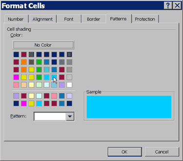
- Choose Sky Blue.
- Click OK. The background of cell B1 is now Sky Blue.
Alternate Method: Adding Background Color by Using the Icon
- Select cells B7 to D7.
- Click the down-arrow next to the Fill Color icon
 .
.
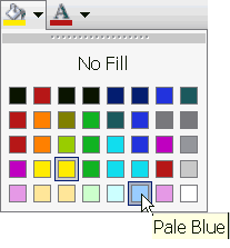
- Select Pale Blue. The background of cells B7 to D7 is now Pale Blue.
Using Auto Format
You can format your data manually or you can use one of Microsoft Excel's many AutoFormats.
- Select cells B1 to D7.
- Choose Format > Auto Format from the menu. Several formats are listed from which you can choose.
- Choose the Accounting 2 format.
- Click OK. Your data is formatted in the Accounting 2 style.
Saving Your File
To save your file:
- Choose File>Save from the menu.
- Go to the directory in which you want to save your file.
- Type lesson2 in the File Name field.
- Click Save.
Closing Microsoft Excel
This is the end of Lesson 2. Close Microsoft Excel.
- Choose File > Exit from the menu.